Efficient Time Interval Stabbing

Introduction

A while back at my job, we needed a solution for splicing together multiple databases seamlessly, with the database user being blissfully unaware this is happening. The discussion of how and why we were doing this are out of scope for this post. Rather, I’ll discuss one subproblem which I found particularly interesting:
given a user’s query time range [start, end], which databases contain data within that time range?

Database Splicing

I’m going to gloss over the details of the database splicing to get to the meat faster. Essentially, existing code would read/write a single database. But wouldn’t it be nice if we could chop up the database as it gets bigger and start a new one? Turns out it would, so we did that and made the existence of these smaller databases transparent to the user so that all data from the past is accessible simply by passing a query time. And even though a system only writes to a single database at a time, it can read from many, including data dropped in from elsewhere.

Requirements for the System

• Databases have a start and end time
• Only one database can be actively written to at a time per machine, but other data can be dropped in place
• Minimal latency is the primary concern
• Minimal memory usage is a secondary concern (assumed to have ample)

The Stabbing Problem

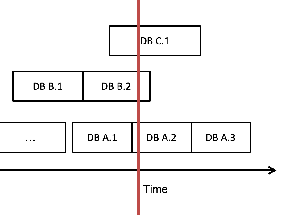
That leads us to the main point, and no it’s not in regards to a rampant serial killer! The stabbing problem mentioned in research literature ¹ involves finding all numerical intervals in a set that a given value “stabs” (is contained by). A corollary of the problem is to find all intervals that overlap with a query range (infinite stabs??). This maps to our database splicing domain when we need to answer the question “which databases should I query in order to find data at time t”? We don’t want to search through all of them because there could be a lot. Let’s use the below example set of databases; note that due to constraints outlined above, databases generated by the same machine can never overlap each other, but data copied in can overlap. If the red line is the stabbing point at time t, then databases A2, B2, and C1 are all going to get stabbed! In other words, those databases contain data at time t.

Storage

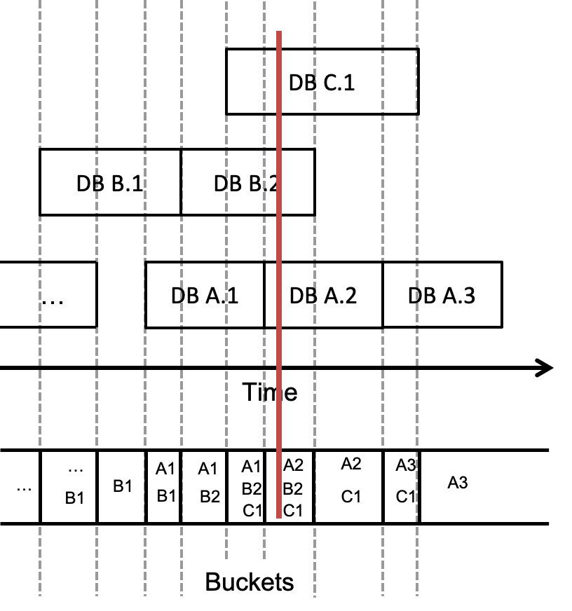
The figure below shows the example database layout that has now been modeled in a storage structure. Each unique endpoint (start or end) of a database marks a new bucket in the storage array, for a total of O(2n) where n is the number of databases. Each bucket then holds pointers to all databases overlapping its time boundaries. This means that a database can exist within 1 or more buckets, and each bucket can contain 0 or more databases. A given time t overlaps the bucket at position p if t >= times[p] and t < times[p+1]. End times are exclusive, so that any time overlaps one and only one time bucket. The end time of the last bucket is defined as positive infinity, so that the active database is within the most recent bucket. In the figure, the dotted gray lines indicate how endpoints contribute to defining the buckets in the storage. The red line is again the stabbing point, and so we can see in the matching bucket at the bottom the resulting set of overlapping databases: A2, B2, and C1.

An alternative approach would be to discretize time into small chunks and then use an array or hash map, so that lookup of a time would be in strictly constant-time. However, this has the downside that the amount of memory used is greatly increased, as well as the time needed to deduplicate intervals in a time range query.

Database Lookup Algorithm

Let’s get to stabbing! What’s the best way to solve this problem given the requirements and constraints?

The Losers

Ideally the query would be constant-time, but this is difficult given that time is a continuous variable. As discussed above, discretizing time into smaller chunks to make it hash-able is appealing given its ability for constant-time lookup, but has multiple disadvantages that make that solution less than ideal.

Given the relatively low number of databases in the typical case, a simple linear search algorithm could be considered, but it’s important to lower the query latency as much as possible and so this is also undesirable.

Many of the accepted solutions in the literature involve balanced binary (interval) trees or skip lists ². A binary tree or skip list is not appropriate for this application because the traversal time of O(lg n) is not fast enough. Furthermore, most additions to the structure will come at the back end as time moves forward, and binary trees provide poor performance when inserts are not randomly distributed.

Another alternative which is commonly used for data indexing in databases is a B-tree ³. This balanced binary tree structure allows for packing many neighboring nodes into the same memory page, which reduces the number of page faults for queries using that index and thus is very performant in practice. This application, though, is less concerned with reducing page faults because the number of databases is likely to be low enough to fit within one or two pages.

First Stab: Binary Search

Ba dum tss. Using the data structure above, finding all databases overlapping a particular time can be accomplished with an interval-based binary search. In this modified form of the search algorithm, query times are checked against the bounds of the candidate time range, then the candidate interval is halved to the left or right based on the comparison. Since intervals cannot overlap and in fact are completely contiguous, the algorithm is guaranteed to return one and only one time-interval bucket. This will lead to a time complexity of O(lg n) ⁴, which is no better than the binary tree traversal.

Optimization: Time Interpolation Search

However, this can be improved with the knowledge that time is always linearly increasing and new databases are created at fairly regular intervals, and therefore the distribution of the bucket endpoints will very likely be roughly uniform. Instead of choosing a candidate bucket in the exact middle of the remaining interval, a better estimate can be made by choosing the bucket that is proportionally located where the target time falls within the range.

As an analogy, this approach is akin to opening a dictionary towards the back when looking for a word starting with ‘w’ instead of in the middle, because it’s expected that words will be roughly evenly distributed throughout (even though this is obviously not strictly true) and ‘w’ is near the end of the alphabet range.

For example, consider the set of buckets [10-30, 30-40, 40-65, 65-75, 75-90], and a target time of 70. The traditional binary search approach would choose the midway point of the range, (40-65). 70 is greater than that range, so another iteration will be taken with the right half of the remaining range [65-75, 75-90], where it will then likely choose the correct range of (65-75). In contrast, the time interpolation search algorithm chooses its candidates with the below equation, which results in the 0-indexed array location to inspect. Immediately, the interpolation search algorithm chooses the correct interval bucket that the target falls in. It will be empirically shown below that this is not an uncommon occurrence.

Python Implementation

Below is some Python code for the intervalInterpolationSearch function described above. End times of buckets are exclusive so that a time will overlap only one bucket. Since the boundary conditions are checked up front in the function, and there are no gaps in time within the bucket structure, the function is guaranteed to find the one and only overlapping bucket for the given time.

def intervalInterpolationSearch(Time[] starts, Time search):
	# Check boundary conditions
	if starts.empty() or search < starts[0]:
		return -1

	if search > starts[-1]
		return len(starts)-1

	lhs = 0, rhs = starts.size()-1, target = -1
	starts.append(Time.now())

	while lhs < rhs and \
			search >= starts[lhs] and \
			search < starts[rhs+1]:
		# Percent of total range where search falls
		ratio = (search-starts[lhs]) / (starts[rhs+1] - starts[lhs])
		# Convert percentage to location within range
		target = lhs + floor(ratio * (rhs - lhs))

		if (search < starts[target]):
			rhs = target - 1 # Iterate with left group only
		elif search >= starts[target + 1]:
			lhs=target+1 # Iterate with right group only
		else:
			break # time is within the target bucket
	return target

Complexity Analysis

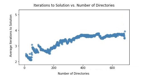
The complexity of interpolation search when the data is uniformly distributed has been shown to be O(lg lg n) ⁴, which for the purpose of keeping track of database directories is near enough to constant-time. This relationship can be seen empirically in the figure below where a sample database distribution was taken from a real system and stored in the format described. Times in between the search boundaries were pulled from a pseudorandom uniform distribution, and the average number of loop iterations needed to get to a solution was plotted. Number of iterations was used as an approximation for performance, because gathering reliable system timing numbers at such a small scale is difficult. As the number of directories used increases, the scatterplot shows the number of iterations needed resembles an O(lg lg n) distribution, staying below 4 for a database set of size 600.

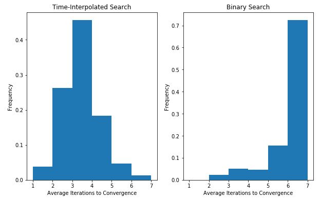
The modified interpolation search was also compared to a typical binary search implementation by performing both algorithms on a directory set of size 100 and a given time chosen from a pseudorandom uniform distribution. This was done for several iterations, and the average number added to a histogram, as per the Statistical Bootstrap Method of garnering statistics about a distribution via resampling ⁵. The chart below shows that utilizing the prior knowledge to perform time-interpolation search vastly improves the number of iterations needed to reach a solution over binary search. It not only seemingly halves the average, but also shifts the whole distribution from being heavily skewed to the right, to being more normal-shaped.

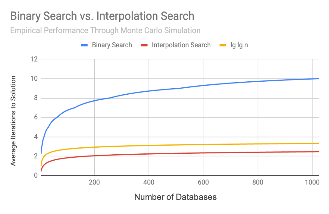
Finally, a Monte Carlo simulation was performed by generating a pseudorandom set of intervals of increasing size and searching for a pseudorandom value one million times. The number of iterations needed to find the correct solution was averaged together across all tests. This was done for both regular binary search and time-interpolation search. Again it can be seen that binary search increases in time at a faster rate than interpolation search, which closely tracks the reference lg(lg n)) plot.

Acknowledgements

Thanks to Chris at null program for the Monte Carlo simulation.

References